Using Attribute Clustering to Improve Compression, Response Time and CPU Consumption: 2. An Example

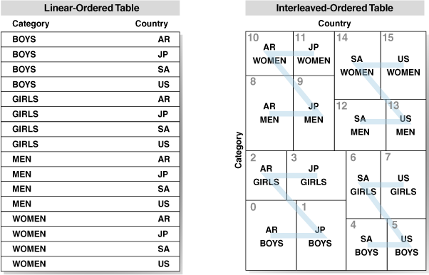
Attribute Clustering reorders data in a table so that similar data values are clustered together.  This can improve both basic and columnar compression, resulting in better response time and lower CPU consumption.

This is the second of a two-part blog post.

1. Introduction
2. Example and Test Results

An Example of Attribute Clustering

This test illustrates the potential benefits of attribute clustering (the scripts are available on GitHub). It simulates the fact table in a data warehouse, or in my use case the General Ledger table in a Financials system. The table will have 20 million rows. Each dimension column will randomly have one of 256 distinct values, padded to 8 characters.  In this case, the distribution of data values is skewed by the square root function.  The alternative commented section produces uniform data. 

create table t0(a varchar2(8 char), b varchar2(8 char), c varchar2(8 char), x number);
truncate table t0;
BEGIN
  FOR i IN 1..2 LOOP
    insert  /*+APPEND PARALLEL*/ into t0
    select  /*+PARALLEL*/
/*--------------------------------------------------------------------------------------------------------------
            rPAD(LPAD(LTRIM(TO_CHAR(FLOOR(dbms_random.value(0,255)),'XX')),2,'0'),8,'X') a
    ,       rPAD(LPAD(LTRIM(TO_CHAR(FLOOR(dbms_random.value(0,255)),'XX')),2,'0'),8,'X') b
    ,       rPAD(LPAD(LTRIM(TO_CHAR(FLOOR(dbms_random.value(0,255)),'XX')),2,'0'),8,'X') c
--------------------------------------------------------------------------------------------------------------*/
            rPAD(LPAD(LTRIM(TO_CHAR(FLOOR(SQRT(dbms_random.value(0,65535))),'XX')),2,'0'),8,'X') a
    ,       rPAD(LPAD(LTRIM(TO_CHAR(FLOOR(SQRT(dbms_random.value(0,65535))),'XX')),2,'0'),8,'X') b
    ,       rPAD(LPAD(LTRIM(TO_CHAR(FLOOR(SQRT(dbms_random.value(0,65535))),'XX')),2,'0'),8,'X') c
--------------------------------------------------------------------------------------------------------------*/
    ,       dbms_random.value(1,1e6)
    from dual connect by level <= 1e7;
    COMMIT;
  end loop;
end;
/
exec dbms_stats.gather_table_stats(user,'T0');

I will create an identical materialized view on that table

create table mv(a varchar2(8 char), b varchar2(8 char), c varchar2(8 char), x number);
create materialized view mv on prebuilt table enable query rewrite as select * from t0;

For each test, I can set different attributes and then fully refresh the materialized view in non-atomic mode.  The various attributes take effect as the materialized view is truncated and repopulated in direct-path mode.

truncate table MV drop storage;
--------------------------------------------------
rem set compression
--------------------------------------------------
--alter materialized view MV nocompress;
--alter materialized view MV compress;
alter materialized view MV compress for query low;
--------------------------------------------------
rem set in memory
--------------------------------------------------
alter table mv inmemory;
--------------------------------------------------
rem set clustering and number of clustering columns
--------------------------------------------------
alter table mv drop clustering;
--alter table mv add clustering by interleaved order (b);
alter table mv add clustering by interleaved order (b, c);
--alter table mv add clustering by interleaved order (b, c, a);
--------------------------------------------------
exec dbms_mview.refresh('MV',atomic_refresh=>FALSE);
exec dbms_inmemory.repopulate(user,'MV');

Then I can see how large the physical and In-Memory segments are.

select * from user_mviews where mview_name = 'MV';
select table_name, tablespace_name, num_rows, blocks, compression, compress_for, inmemory, inmemory_compression 
from user_tables where table_name IN('MV','T0');
select segment_name, segment_type, tablespace_name, bytes/1024/1024 table_MB, blocks, extents, inmemory, inmemory_compression
from user_Segments where segment_name IN('MV','T0');

with x as (
select segment_type, owner, segment_name, inmemory_compression, inmemory_priority
, count(distinct inst_id) instances
, count(distinct segment_type||':'||owner||'.'||segment_name||'.'||partition_name) segments
, sum(inmemory_size)/1024/1024 inmemory_mb, sum(bytes)/1024/1024 tablespace_Mb
from   gv$im_segments i
where segment_name = 'MV'
group by segment_type, owner, segment_name, inmemory_compression, inmemory_priority)
select x.*, inmemory_mb/tablespace_mb*100-100 pct from x
order by owner, segment_type, segment_name
/

I will use a simple test query to see how the performance changes

select b,c, count(a), sum(x) from t0 where b='2AXXXXXX' group by b,c fetch first 10 rows only;

I tested 

• Uniformly distributed data -v- skewed data
• Without table compression -v- basic compression -v- Hybrid Columnar Compression (HCC)
• No attribute clustering -v- interleaved clustering on 1, 2, and 3 columns

Table      Tablespace                                                                                         
Name       Name         NUM_ROWS     BLOCKS COMPRESS COMPRESS_FOR                   INMEMORY INMEMORY_COMPRESS
---------- ---------- ---------- ---------- -------- ------------------------------ -------- -----------------
MV         PSDEFAULT    20000000      60280 ENABLED  QUERY LOW                      ENABLED  FOR QUERY LOW    
T0         PSDEFAULT    20000000     150183 DISABLED                                DISABLED                  

                      Tablespace      Table                                                 
Segment Na Segment Ty Name               MB     BLOCKS    EXTENTS INMEMORY INMEMORY_COMPRESS
---------- ---------- ---------- ---------- ---------- ---------- -------- -----------------
MV         TABLE      PSDEFAULT       472.0      60416        130 ENABLED  FOR QUERY LOW    
T0         TABLE      PSDEFAULT     1,220.0     156160        203 DISABLED                  

                                                                                 In Memory Tablespace           
Segment Ty OWNER    Segment Na INMEMORY_COMPRESS INMEMORY  INSTANCES   SEGMENTS         MB         MB        PCT
---------- -------- ---------- ----------------- -------- ---------- ---------- ---------- ---------- ----------
TABLE      SYSADM   MV         FOR QUERY LOW     NONE              2          1      829.2      936.6 -11.4662752

With query rewrite on the materialized view and the materialized view in the In-Memory store, we see Oracle rewrite the query from the underlying table to the materialized view and then to an in-memory query.

select b,c, sum(x) from t0 where b='2AXXXXXX' group by b,c;

Plan hash value: 389206685
-----------------------------------------------------------------------------------------------
| Id  | Operation                              | Name | Rows  | Bytes | Cost (%CPU)| Time     |
-----------------------------------------------------------------------------------------------
|   0 | SELECT STATEMENT                       |      |   182 |  7280 |   876  (31)| 00:00:01 |
|   1 |  HASH GROUP BY                         |      |   182 |  7280 |   876  (31)| 00:00:01 |
|*  2 |   MAT_VIEW REWRITE ACCESS INMEMORY FULL| MV   | 78125 |  3051K|   875  (31)| 00:00:01 |
-----------------------------------------------------------------------------------------------

Test Results

Conclusions

• Without any table compression, attribute clustering does not affect the size of the table on the tablespace, but the size of the table in the In-Memory store is reduced, and query performance is improved.
• With either basic or Hybrid Columnar compression, attribute clustering reduces the size of the table both in the tablespace and in the in-memory store.
• All forms of compression and attribute clustering increase the duration of the materialized view refresh. Degradation of the refresh due to clustering was less severe with HCC than with either no compression or simple compression.
• I found that query performance degraded when using interleaved clustering in combination with simple compression although this resulted in a smaller in-memory segment than HCC, but performance improved with HCC.
• Uniform data compressed marginally better than skewed.  Otherwise, they produced very similar results.  
• You do not have to take advantage of compression on the physical segment to take advantage of the compression in In-Memory, but you may get better performance if you do.
• With this test data set, optimal performance was achieved when clustering on 2 dimension columns. When clustering on all three columns I obtained worse compression and query performance. This varies with the data. With real-world data, I have had examples with better compression and performance with the maximum of 4 clustering column groups. Generally, the best performance corresponds to the attribute clustering that gives the best columnar compression. This is not always the case for simple compression.

Using Attribute Clustering to Improve Compression, Response Time and CPU Consumption: 1. Introduction

Attribute Clustering reorders data in a table so that similar data values are clustered together.  This can improve both basic and columnar compression, resulting in better response time and lower CPU consumption.

This is the first of a two-part blog post.

1. Introduction
2. Example and Test Results

Use Case

I am working on a Financials system running on an engineered system.  It runs a daily batch of GL reports on summary ledgers that have unindexed materialized views.  The materialized views are also hybrid column compressed (HCC) to reduce their size and improve reporting performance.  

We also put the materialized views into the In-Memory store.  Initially, we used 'free' base-level In-Memory and worked within the 16Gb/instance limit.  Having moved to Exadata Cloud@Customer, we can use the fully licensed version of In-Memory.

Now I have introduced Attribute Clustering for the materialized views.

Attribute Clustering

Attribute Clustering has been available on Enterprise Edition since Oracle 12.1.0.2.  Data is clustered in close physical proximity according to certain columns.  Linear Ordering stores the data according to the order of the specified clustering columns.  Interleaved Ordering uses a Z-order curve to cluster data in multiple dimensions (this graphic is from Oracle's documentation).

The GL reports have multiple combinations of different predicates. Therefore, as recommended by Oracle, we used interleaved ordering.  Linear ordering is not suitable in this case because there is no single suitable order for each table.  Linear ordering also caused the runtime of the materialized view refresh to extend much more than interleaved ordering as it has to sort the data.

We have not introduced Zone Maps.  That is to say that after testing, we removed them.  Zone maps can be thought of as a coarse index of the zones in the attribute clustering, and would normally be expected to improve the access of the data.  You can see them being used in the execution plans to access the table both in the tablespace and in the In-Memory store.  However, our application dynamically generates a lot of SQL and therefore performs a lot of SQL parse.  We found that the additional work to process the zone map significantly degraded performance.

Attribute Clustering is not enforced for every DML operation. It only affects direct-path insert operations, data movement, or table creation. It is easy to implement it for segments that are already HCC, which also relies on direct-path operations.  The materialized views were created to introduce HCC, hence they are refreshed in non-atomic mode which truncates and repopulates them in direct-path mode.  Thus attribute clustering specified on the materialized views will be implemented as they refresh.

Historical, and therefore static, partitions in the ledger tables are marked for HCC, and we schedule an online rebuild to compress them.  Now, that will also apply attribute clustering.  This process could be automated with Automatic Storage Compression.

Compression

Simply by storing similar data values together, we obtained better compression from HCC.  The tables underlying the materialized views were smaller.  

In-Memory also uses columnar compression.  Attribute clustering produced a reduction in the size of segments in the In-Memory store.  If we were still working within the constraints of Base-Level In-Memory, we would have been able to store more segments in In-Memory.

We are using attribute clustering not to directly improve data access, but to harness a secondary effect, that of improved compression.  We are seeing a reduction in the runtime of the reports.  Most of the database time is already spent on the CPU (as most of the fact tables are in In-Memory), so this translates to a reduction in CPU consumption.  We can consider running more reports concurrently to complete the batch earlier.  We can also consider reducing the number of CPUs and therefore reduce cloud subscription costs.

The second part of this blog will show an example test script and results.