Using Attribute Clustering to Improve Compression, Response Time and CPU Consumption: 2. An Example

Attribute Clustering reorders data in a table so that similar data values are clustered together.  This can improve both basic and columnar compression, resulting in better response time and lower CPU consumption.

This is the second of a two-part blog post.

1. Introduction
2. Example and Test Results

An Example of Attribute Clustering

This test illustrates the potential benefits of attribute clustering (the scripts are available on GitHub). It simulates the fact table in a data warehouse, or in my use case the General Ledger table in a Financials system. The table will have 20 million rows. Each dimension column will randomly have one of 256 distinct values, padded to 8 characters.  In this case, the distribution of data values is skewed by the square root function.  The alternative commented section produces uniform data. 

create table t0(a varchar2(8 char), b varchar2(8 char), c varchar2(8 char), x number);
truncate table t0;
BEGIN
  FOR i IN 1..2 LOOP
    insert  /*+APPEND PARALLEL*/ into t0
    select  /*+PARALLEL*/
/*--------------------------------------------------------------------------------------------------------------
            rPAD(LPAD(LTRIM(TO_CHAR(FLOOR(dbms_random.value(0,255)),'XX')),2,'0'),8,'X') a
    ,       rPAD(LPAD(LTRIM(TO_CHAR(FLOOR(dbms_random.value(0,255)),'XX')),2,'0'),8,'X') b
    ,       rPAD(LPAD(LTRIM(TO_CHAR(FLOOR(dbms_random.value(0,255)),'XX')),2,'0'),8,'X') c
--------------------------------------------------------------------------------------------------------------*/
            rPAD(LPAD(LTRIM(TO_CHAR(FLOOR(SQRT(dbms_random.value(0,65535))),'XX')),2,'0'),8,'X') a
    ,       rPAD(LPAD(LTRIM(TO_CHAR(FLOOR(SQRT(dbms_random.value(0,65535))),'XX')),2,'0'),8,'X') b
    ,       rPAD(LPAD(LTRIM(TO_CHAR(FLOOR(SQRT(dbms_random.value(0,65535))),'XX')),2,'0'),8,'X') c
--------------------------------------------------------------------------------------------------------------*/
    ,       dbms_random.value(1,1e6)
    from dual connect by level <= 1e7;
    COMMIT;
  end loop;
end;
/
exec dbms_stats.gather_table_stats(user,'T0');

I will create an identical materialized view on that table

create table mv(a varchar2(8 char), b varchar2(8 char), c varchar2(8 char), x number);
create materialized view mv on prebuilt table enable query rewrite as select * from t0;

For each test, I can set different attributes and then fully refresh the materialized view in non-atomic mode.  The various attributes take effect as the materialized view is truncated and repopulated in direct-path mode.

truncate table MV drop storage;
--------------------------------------------------
rem set compression
--------------------------------------------------
--alter materialized view MV nocompress;
--alter materialized view MV compress;
alter materialized view MV compress for query low;
--------------------------------------------------
rem set in memory
--------------------------------------------------
alter table mv inmemory;
--------------------------------------------------
rem set clustering and number of clustering columns
--------------------------------------------------
alter table mv drop clustering;
--alter table mv add clustering by interleaved order (b);
alter table mv add clustering by interleaved order (b, c);
--alter table mv add clustering by interleaved order (b, c, a);
--------------------------------------------------
exec dbms_mview.refresh('MV',atomic_refresh=>FALSE);
exec dbms_inmemory.repopulate(user,'MV');

Then I can see how large the physical and In-Memory segments are.

select * from user_mviews where mview_name = 'MV';
select table_name, tablespace_name, num_rows, blocks, compression, compress_for, inmemory, inmemory_compression 
from user_tables where table_name IN('MV','T0');
select segment_name, segment_type, tablespace_name, bytes/1024/1024 table_MB, blocks, extents, inmemory, inmemory_compression
from user_Segments where segment_name IN('MV','T0');

with x as (
select segment_type, owner, segment_name, inmemory_compression, inmemory_priority
, count(distinct inst_id) instances
, count(distinct segment_type||':'||owner||'.'||segment_name||'.'||partition_name) segments
, sum(inmemory_size)/1024/1024 inmemory_mb, sum(bytes)/1024/1024 tablespace_Mb
from   gv$im_segments i
where segment_name = 'MV'
group by segment_type, owner, segment_name, inmemory_compression, inmemory_priority)
select x.*, inmemory_mb/tablespace_mb*100-100 pct from x
order by owner, segment_type, segment_name
/

I will use a simple test query to see how the performance changes

select b,c, count(a), sum(x) from t0 where b='2AXXXXXX' group by b,c fetch first 10 rows only;

I tested 

• Uniformly distributed data -v- skewed data
• Without table compression -v- basic compression -v- Hybrid Columnar Compression (HCC)
• No attribute clustering -v- interleaved clustering on 1, 2, and 3 columns

Table      Tablespace                                                                                         
Name       Name         NUM_ROWS     BLOCKS COMPRESS COMPRESS_FOR                   INMEMORY INMEMORY_COMPRESS
---------- ---------- ---------- ---------- -------- ------------------------------ -------- -----------------
MV         PSDEFAULT    20000000      60280 ENABLED  QUERY LOW                      ENABLED  FOR QUERY LOW    
T0         PSDEFAULT    20000000     150183 DISABLED                                DISABLED                  

                      Tablespace      Table                                                 
Segment Na Segment Ty Name               MB     BLOCKS    EXTENTS INMEMORY INMEMORY_COMPRESS
---------- ---------- ---------- ---------- ---------- ---------- -------- -----------------
MV         TABLE      PSDEFAULT       472.0      60416        130 ENABLED  FOR QUERY LOW    
T0         TABLE      PSDEFAULT     1,220.0     156160        203 DISABLED                  

                                                                                 In Memory Tablespace           
Segment Ty OWNER    Segment Na INMEMORY_COMPRESS INMEMORY  INSTANCES   SEGMENTS         MB         MB        PCT
---------- -------- ---------- ----------------- -------- ---------- ---------- ---------- ---------- ----------
TABLE      SYSADM   MV         FOR QUERY LOW     NONE              2          1      829.2      936.6 -11.4662752

With query rewrite on the materialized view and the materialized view in the In-Memory store, we see Oracle rewrite the query from the underlying table to the materialized view and then to an in-memory query.

select b,c, sum(x) from t0 where b='2AXXXXXX' group by b,c;

Plan hash value: 389206685
-----------------------------------------------------------------------------------------------
| Id  | Operation                              | Name | Rows  | Bytes | Cost (%CPU)| Time     |
-----------------------------------------------------------------------------------------------
|   0 | SELECT STATEMENT                       |      |   182 |  7280 |   876  (31)| 00:00:01 |
|   1 |  HASH GROUP BY                         |      |   182 |  7280 |   876  (31)| 00:00:01 |
|*  2 |   MAT_VIEW REWRITE ACCESS INMEMORY FULL| MV   | 78125 |  3051K|   875  (31)| 00:00:01 |
-----------------------------------------------------------------------------------------------

Test Results

Conclusions

• Without any table compression, attribute clustering does not affect the size of the table on the tablespace, but the size of the table in the In-Memory store is reduced, and query performance is improved.
• With either basic or Hybrid Columnar compression, attribute clustering reduces the size of the table both in the tablespace and in the in-memory store.
• All forms of compression and attribute clustering increase the duration of the materialized view refresh. Degradation of the refresh due to clustering was less severe with HCC than with either no compression or simple compression.
• I found that query performance degraded when using interleaved clustering in combination with simple compression although this resulted in a smaller in-memory segment than HCC, but performance improved with HCC.
• Uniform data compressed marginally better than skewed.  Otherwise, they produced very similar results.  
• You do not have to take advantage of compression on the physical segment to take advantage of the compression in In-Memory, but you may get better performance if you do.
• With this test data set, optimal performance was achieved when clustering on 2 dimension columns. When clustering on all three columns I obtained worse compression and query performance. This varies with the data. With real-world data, I have had examples with better compression and performance with the maximum of 4 clustering column groups. Generally, the best performance corresponds to the attribute clustering that gives the best columnar compression. This is not always the case for simple compression.

Using Attribute Clustering to Improve Compression, Response Time and CPU Consumption: 1. Introduction

Attribute Clustering reorders data in a table so that similar data values are clustered together.  This can improve both basic and columnar compression, resulting in better response time and lower CPU consumption.

This is the first of a two-part blog post.

1. Introduction
2. Example and Test Results

Use Case

I am working on a Financials system running on an engineered system.  It runs a daily batch of GL reports on summary ledgers that have unindexed materialized views.  The materialized views are also hybrid column compressed (HCC) to reduce their size and improve reporting performance.  

We also put the materialized views into the In-Memory store.  Initially, we used 'free' base-level In-Memory and worked within the 16Gb/instance limit.  Having moved to Exadata Cloud@Customer, we can use the fully licensed version of In-Memory.

Now I have introduced Attribute Clustering for the materialized views.

Attribute Clustering

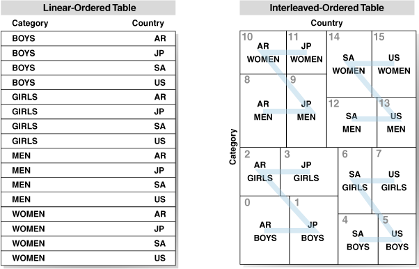
Attribute Clustering has been available on Enterprise Edition since Oracle 12.1.0.2.  Data is clustered in close physical proximity according to certain columns.  Linear Ordering stores the data according to the order of the specified clustering columns.  Interleaved Ordering uses a Z-order curve to cluster data in multiple dimensions (this graphic is from Oracle's documentation).

The GL reports have multiple combinations of different predicates. Therefore, as recommended by Oracle, we used interleaved ordering.  Linear ordering is not suitable in this case because there is no single suitable order for each table.  Linear ordering also caused the runtime of the materialized view refresh to extend much more than interleaved ordering as it has to sort the data.

We have not introduced Zone Maps.  That is to say that after testing, we removed them.  Zone maps can be thought of as a coarse index of the zones in the attribute clustering, and would normally be expected to improve the access of the data.  You can see them being used in the execution plans to access the table both in the tablespace and in the In-Memory store.  However, our application dynamically generates a lot of SQL and therefore performs a lot of SQL parse.  We found that the additional work to process the zone map significantly degraded performance.

Attribute Clustering is not enforced for every DML operation. It only affects direct-path insert operations, data movement, or table creation. It is easy to implement it for segments that are already HCC, which also relies on direct-path operations.  The materialized views were created to introduce HCC, hence they are refreshed in non-atomic mode which truncates and repopulates them in direct-path mode.  Thus attribute clustering specified on the materialized views will be implemented as they refresh.

Historical, and therefore static, partitions in the ledger tables are marked for HCC, and we schedule an online rebuild to compress them.  Now, that will also apply attribute clustering.  This process could be automated with Automatic Storage Compression.

Compression

Simply by storing similar data values together, we obtained better compression from HCC.  The tables underlying the materialized views were smaller.  

In-Memory also uses columnar compression.  Attribute clustering produced a reduction in the size of segments in the In-Memory store.  If we were still working within the constraints of Base-Level In-Memory, we would have been able to store more segments in In-Memory.

We are using attribute clustering not to directly improve data access, but to harness a secondary effect, that of improved compression.  We are seeing a reduction in the runtime of the reports.  Most of the database time is already spent on the CPU (as most of the fact tables are in In-Memory), so this translates to a reduction in CPU consumption.  We can consider running more reports concurrently to complete the batch earlier.  We can also consider reducing the number of CPUs and therefore reduce cloud subscription costs.

The second part of this blog will show an example test script and results.

Practical Application Performance Tuning: Applying Theory in Practice

I gave this presentation at the UKOUG Techfest 19 conference.  It is closely based on a previous presentation about PeopleSoft nVision performance tuning, and uses the experience of a PeopleSoft project as a case study, so I am also posting here and on my PeopleSoft blog.

This video was produced as a part of the preparation for this session.  The slide deck is also available on my website.

Learning about and understanding the principles and mechanics of the Oracle database is fundamentally important for both DBAs and developers. It is one of the reasons we still attend physical conferences.
This presentation tells the story of a performance tuning project for the GL reporting on a Financials system on an Oracle engineered system. It required various database techniques and features to be brought to bear. Having a theoretical understanding of how the database and various features work allowed us to make reasonable predictions about whether they would be effective in our environment. Some ideas were discounted, some were taken forward.
We will look at instrumentation, ASH, statistics collection, partitioning, hybrid columnar compression, Bloom filtering, SQL profiles. All of them played a part in the solution, some were simple and effective, some will require periodic maintenance, some added further complications that had to be worked around, some had to be carefully configured in-line with the application, and some required some reconfiguration of the application into order to work properly.

Choosing the Right Compression

Choosing the right database table compression matters.  It affects the size of the objects and also the performance of your application.  Compression makes objects smaller, and for many systems, this is an objective in itself, but it also affects performance.  As compressed objects are smaller, less physical I/O is required to access them.  However, that saving is paid for in CPU.  More CPU is required to compress the data when it is written, and then again (albeit usually less CPU) to decompress it when you read it.  The question is whether the saving in I/O pays for the additional CPU.

There are a number of forms of compression to choose between.  They have different characteristics.  The resulting objects are different sizes, and they require different amounts of CPU to compress and decompress.

• Basic Compression:  This is not really compression, but a form of block-level de-duplication.  It has been available since Oracle 9i.  It is available on all platforms.
• Hybrid Columnar Compression is only available on Engineered Systems, FS Flash Storage System and ZFS Storage Appliance (ZFSSA).  4 different levels of compression that use 3 different compression algorithms.  HCC is frequently positioned as being highly effective at reducing the size of data warehouses, but it also has implications for performance.
• Query Low: LZO algorithm
• Query High: ZLIB algorithm
• Archive Low: ZLIB algorithm higher level with a larger block size.
• Archive High: BZIP2 algorithm.  The higher compression ratio comes at the expense of significantly increased CPU overhead on decompression.

Further Reading:

• If you are not familiar with the various forms of compression, and their licencing requirements, then Franck Pachot’s blog Oracle compression, availability and licencing will set the scene.
• As early as 2016, Roger MacNichol pointed out in Compression in a well-balanced system that “since HCC was released …, DBAs have almost always used Query High” but as CPU speeds have increased “the time has come for a reassessment of role HCC Query Low”.  This blog relates such a case in point.
• Oracle White Paper: Hybrid Columnar Compression (HCC) on Oracle Database 18c 

Which one is right for your application?  It depends.  Ultimately, you need to test it for yourself.  In this blog, I am going to relate my experience of one particular system, including how I tested it.  Our objective was optimising performance, rather than reducing database size.

My Test System

• SuperCluster M7 (i.e. an Engineered System), Oracle 12.1.0.2, 2-node RAC, running PeopleSoft Financials 9.2.
• In particular, this system runs a large number of complex PeopleSoft General Ledger nVision reports that use a number of reporting views on summary ledgers. There are materialized views built on the reporting views.  The summary ledgers are updated nightly.  Then the materialized views are fully refreshed in non-atomic mode so the tables are truncated and repopulated in direct-path mode.  Hence, they can be Hybrid Columnar Compressed without needing the Advanced Compression licence.  The materialized views are not indexed.  Thus they can only be full scanned, and these scans can be offloaded to the storage cells (i.e. smart scan).

The metrics presented here are extracted from test system where the summary ledger tables are updated, materialised view refreshed and then 136 General Ledger (GL) report books are run on regular a daily schedule.  This approach ensures that each test is, as far as was possible, run with the same initial conditions and only known parameters are changed each time.  In each test, a different compression level was set on the materialized views.

• I have not investigated ARCHIVE compression.

Writing

Description	Materialized Views
	Size (MB)	Comp. %	Comp. Ratio	Elapsed	Total DB Time
No Compression	151,868	0%	1.0	1:01	18:13
Basic Compression	34,720	77%	4.4	1:12	22:54
Query Low	22,666	85%	6.7	1:00	18:27
Query High	14,086	91%	10.8	1:05	22:56

all times expressed in hours:minutes

• While basic compression does significantly reduce table sizes (4.4x), Hybrid Columnar Compression does better (6.7x – 10.8x).  
• HCC Query Low only has a very small overhead while writing data.  The materialized views are refreshed in parallel, and while the total DB time is higher, the elapsed time is lower!
• Both basic compression and HCC Query High take about 20% longer to write the data in direct path mode.

Reading

Description	nVision DB Time
	On CPU+CPU Wait	cell smart table scan	Others	Total	On CPU+CPU Wait	cell smart table scan	Others
No Compression	201:26	97:12	18:15	316:54	64%	31%	6%
Basic Compression	466:13	66:03	31:07	563:24	83%	12%	6%
Query Low	241:13	12:34	44:57	298:45	81%	4%	15%
Query High	278:20	4:43	11:38	294:42	94%	2%	4%

The nVision GL reports only read the materialized views (although they do write some temporary working storage tables).

• As the level of compression of the materialized views increases, the time spent on cell smart table scan (physical read) decreases, this is mainly because the objects are smaller.
• The slightly surprising result is that the CPU overhead of basic compression is higher than either form of HCC, and more than twice that of using uncompressed tables.  Hence it significantly increases the total database response time
• Both forms of query HCC perform better than the uncompressed table.  The increase in CPU time is more than compensated by the reduction in time spent on physical I/O.
• The Query low test was affected by other factors external to the test (a lot more time spent in other wait events).  Otherwise, it would have outperformed query high.  If we look at just CPU and physical read time it is clearly the best option.

In an offloaded (i.e. smart) scan on an engineered system, decompression as well as the physical I/O is done in the storage cell.  The saving in time spent on physical between query low and query high is small because the disk subsystem performs so well on the engineered system.
Whereas on a non-engineered system compression and I/O must be done by the database server, there is nowhere else.  You may well find that a different level of compression is optimal.

Conclusion

• Basic compression exhibits a surprisingly high CPU overhead.  In my test, the performance was poorer than with uncompressed tables.
• HCC Query low was generally the best option, saving in I/O more than paid for the increase in CPU.  
• I also analysed ASH data for the different tests broken down by materialized view.  I found it was better to leave smaller materialized views uncompressed but to compress the larger ones.  This is not surprising since HCC adds additional structures.

These results and conclusions are from one set of test on one particular application, on one particular 'engineered' hardware configuration using one particular data set.  So you need to conduct your own comparative test and decide what is best for your system.